Intro
Regularization techniques are useful in helping combat the problem of overfitting. In this article, I will be implementing and going in depth on Lasso Regression (L1 regularization) and Ridge Regression (L2 regularization). Before we start, regularization techniques require the knowledge of two main concepts - overfitting and the loss function.
Overfitting
Models that are overfitting will generalize too specifically to the training data, and return poor performance on new sets of data. The issue at hand is that the model is constructed in such fashion that it captures all the noise and patterns within the training data. This may be beneficial, if new data show similar trends and patterns as the training data. However, in many instances this is not the case. A model that fits too tightly to the training data will often perform poorly on a new set of data. In order to make accurate predictions, one must avoid overfitting and achieve a model that generalizes well to new data.
Loss Function
Let’s take a look at an OLS linear regression problem. In this made up example, let’s say we’re predicting temperature based off of humidity levels, amount of wind, and precipitation levels. The model is constructed such that the coefficient estimates for wind, humidity, and precipitation will minimize the Sum of Squared Residuals. This is actually calculated in what’s called the loss function.
Within the loss function, multiple predicted values are tried for the coefficients. The first set of predicted values are constructed, and the Sum of Squared Residuals is returned. In an iterative fashion, another set of predicted coefficients is tried, again returning a score of SS Residuals. This process is done until the SS Residuals is minimized. The coefficients in the final model will be the one that minimizes this loss function.
Regularization
By minimizing the Sum of Squared Residuals, the model, by nature, is designed to optimally fit the training data. However, like I mentioned above, this model is now designed specifically for the training data and may not generalize well to new data.
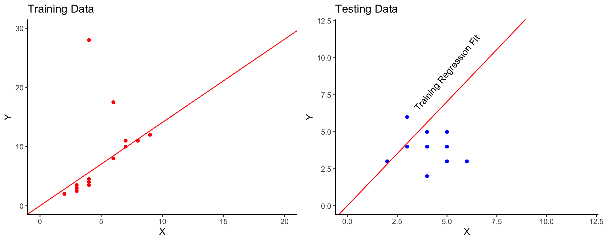
Let’s take a look at an example. Let’s say we have a few data points for the training data and fit a linear regression to it.

Notice how in the training data we have higher values and an outlier point. The linear regression is fit to match this data to the best of it’s ability, so that outlier will have an impact on the fit. Now look at the testing data. In the testing data, we do not see those larger values. The fit from the training data does not extend to the testing data very well. Actually, the fit is quite bad.
Regularization techniques are designed to sacrifice this optimal fit to the training data to gain a better generalization to new data. In simpler terms, this is basically sacrificing the complex, strict model for a model that is more robust and flexible.
L1 and L2 regularization methods put a constraint on the predicted coefficients by allowing the user to set a term of \(\lambda\). \(\lambda\) is essentially a term that penalizes coefficients for being too large. When \(\lambda\) is 0, no difference is observed between the original model and the new regularized model. As \(\lambda\) increases, a higher emphasis is setting on lowering the coefficients. In machine learning terms, \(\lambda\) increases with bias, and \(\lambda\) decrease with variance.
Bias helps the model generalize better, putting less emphasize on noisy, single points. If the bias is too high, the model will be underfitting. Variance is the opposite of bias, referring to a models sensitivity to noisy points. If the variance is too high, the model will overfitting. The goal when fitting models is to find the perfect balance between bias and variance. Easier said then done, most of the time.
Ridge Regression (L2 Regularization)
Whereas in classic linear regression, the loss function may be the calculation of Sum of Squared Residuals, the new loss function now includes the addition of the coefficient estimates. These coefficients are attached to the weight, \(\lambda\). The idea behind this is that now, large coefficients will return higher scores on the loss function. If the goal is to minimize this loss function, large coefficients are essentially “penalizing” the model. And remember, smaller coefficients tend to return more robust models. Specifically, the loss function is now designed as the residuals plus lambda times the sum of of squared coefficient estimates.
Therefore, the specification of \(\lambda\) will allow the user to play around with the bias and variance of the model. This is particularly of use when your model may contain a large amount of variables that are noisy, or that don’t contribute much information in regards to the response variable. Ridge Regression can set lower coefficient values for these unimportant variables, pushing them closer to zero. Ridge regression can push coefficients close to zero, but not entirely there.
Lasso Regression (L1 Regularization)
The name Lasso stands for Least Absolute Shrinkage and Selection Operator. Lasso Regression operates in a pretty similar fashion to Ridge Regression. The main idea is to reduce the magnitude of the coefficients to achieve a more robust model. However, in Lasso Regression, coefficients can be pushed to zero. Essentially, this removes the attached variable out of the equation, acting as a form of feature selection.
Lasso regression again uses the term of \(\lambda\) as a hyperparameter to allow the user to control bias and variance. The loss function for Lasso Regression is identical to Ridge Regression, differing only in the fact that Lasso Regression drops the square on the coefficients and just takes the absolute value. So the loss function is now the sum of squared residuals plus lambda times the sum of the absolute values of the estimated coefficients.